Example Gallery
You may check out a short description of some of the examples detailed in the manualDocument reading. Each of them was generated by a few lines script, which are provided with the software together with extensive comments.
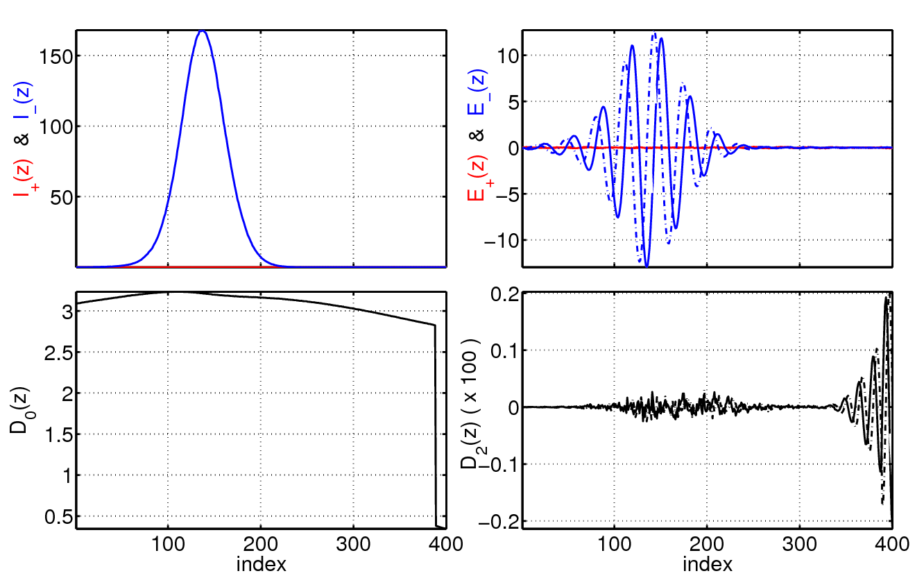
Multimode Dynamics
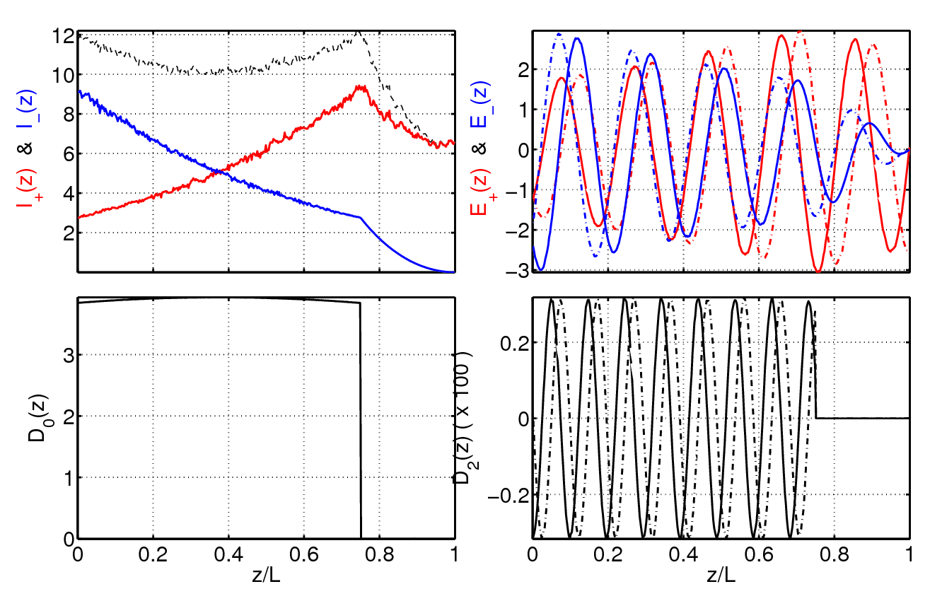
Among the possible problems that Freetwm can tackle, it can be used to study the multimode dynamics of semiconductor laser diodes out of the uniform field limit, a domain where very few theoretical results exist, although it is in this regime that most semiconductor lasers operate. As an example, one can observe on the right some typical results of multimode dynamics obtained for a Fabry-Perot laser in which the left facet has a high reflectivity while the right facet is anti-reflection treated. As a result of the large cavity losses, one obtains a strongly spatially asymmetric profile both for the field and the carrier density distribution (D0) within the cavity (see bottom left). In addition, the model takes into account the influence of spatial hole burning (D2) in the active material gain created by the interference pattern between the counter-propagating fields which act as a important source of gain saturation, (see bottom right).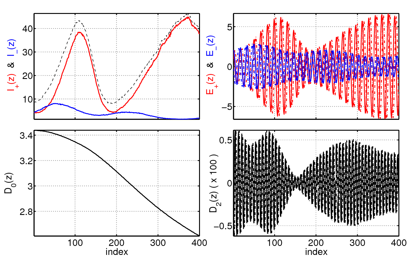
Optical Injection
The response of an optical system to external injection of light is a very important topic in photonics. Freetwm can be used to study the optical response of active devices subjected to arbitrary forms of optical injections. Here we exemplify the case of a ring laser which can operate into a bistable unidirectional regime and may be used as an optical latch. A sufficiently intense light injection can trigger a reversal of the direction of emission, see for instance [5,7]. On the left, one can observe the dynamical response of the ring submitted to a 1 ns quasi-square optical pulse. The black filling represents actually the carrier wave frequency of the square pulse. Upon releasing the injection the direction of emission persists, after some transient relaxation oscillations where the intensity and the carrier reservoir reach equilibrium. The initial condition for the right panels is given by the final state of the time evolution on the left panels. Such states can be conveniently saved and loaded in binary mat files allowing for easy parametric studies.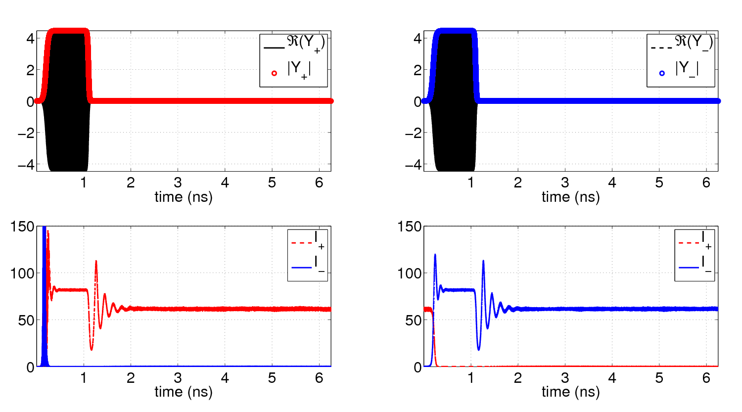
Distributed Feedback
Distributed Feedback lasers and Distributed Feedback Gratings can also be modeled by simply creating an arbitrary index profile within the cavity, like it is showed on the picture below on the left. The spatial oscillation represents the offset of the Bragg wavevector with respect to the semiconductor band-gap taken here as a reference. Here the oscillation is purely harmonic signaling the absence of chirp within the grating. One can see the influence of the index grating on the right figure as it acts as a distributed reflector for the field amplitudes.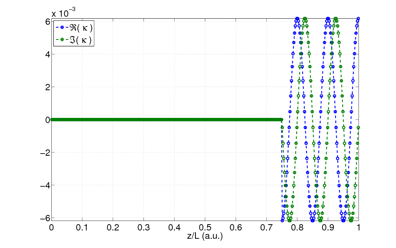
Passive Mode-Locking
One the primary objective of Freetwm is the study of Passive Mode-Locking in the presence of reverse biased saturable absorber, like e.g. in [5, 9]. Doing so is therefore very easy and can be achieved by imposing different optical properties in different sections of the laser cavity, like e.g. a fast voltage induced sweep-out rate of the optically generated carriers or an offset of the semiconductor band-gap wavelength due to the Quantum confined Stark effect. For appropriate parameters, one can trigger the onset of pulsating mode-locked regime. One can see on the right picture the pulsating amplitude of the field at both output facets as well as the characteristic evolution of the population inversion (D0) in the gain and within the absorber sections. The strong peak in the RF power spectrum at the modal separation signal fundamental Mode-Locking as well as the residual contribution of the relaxation oscillations around 5 GHz. The setup of such a photonic device can be achieved in several ways, e.g. by assuming spatially dependent optical properties or by defining a device composed of several sections, each one possessing uniform optical properties. These sections are then coupled only at the level of the boundary conditions which in the simplest case is a transmission matrix but can also contain the effect of some residual reflectivities at the gain-absorber junction. NB: the animation from the starting page was generated from the final state of this simulation.
Delay Equation Mapping
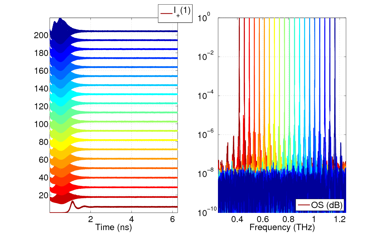
One can obtain a very important speedup by using the option of mesh decimation. Decimation consists in replacing D points of the mesh by the analytical solution of the wave equation with source. This is done starting from the first point on the left of the cavity toward the last one on the right side. This transformation is done by replacing the traveling wave equations by coupled Delay Algebraic Equations (DAE), see [2] for details. For the sake of simplicity, we consider here a situation similar to the one described in the previous example of Passive Mode-Locking, namely a two section Fabry-Perot laser with a short saturable absorber section. As we are free to choose different decimation factors in each section, we denote in the following D1 and D2 the decimation factors in the gain and the absorber section, respectively. The discretization for the two sections is (N1,N2) = (513, 17). One can see on the left the time trace for the output intensity on the right facet of the absorber section. From top to bottom, the decimation factors are: (D1, D2) = (1, 1) (no decimation), (D1, D2) = (16, 2), (D1, D2) = (32, 4) and (D1, D2) = (32, 8), respectively. figure ExampleG_1.png Notice that although the transient are, and must be, different, the steady state regime and the predicted pulsewidth are identical. The speedup in the bottom case as compared to the top one is close to 40. This approach allows to bridge time consuming spatially distributed model with the much less resource hungry delay equation approach. The option of decimation is available only if the mesh lengths N is odd and such that (N − 1)⁄D is a natural number . Finally, if one use power of two for N − 1 and D, each mesh is a subset of the previous one which allows restarting the simulation from the previous ones to study the accuracy of the truncation for increasing values of D.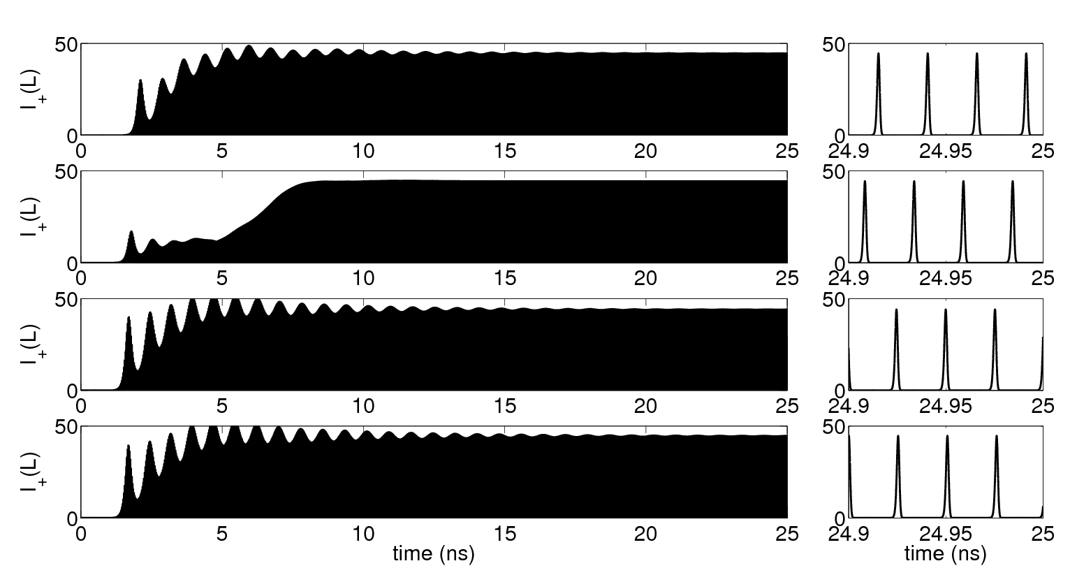
Intracavity Features
Compound cavity lasers have very interesting properties due to the interference between modal combs. The so-called Vernier effect may induce either strongly monomode dynamics or high frequency modal beating, see for instance [8]. This type of dynamics can be studied with Freetwm following a versatile approach: for a low number of intracavity reflectors, one can define several sub-sections, coupled via their respective boundary conditions. However, when the number of intracavity reflector is large, like e.g. to form a rough photonic crystal, this approach is not practical and we provide another method where one can insert directly reflectors inside a single section. On the left, one can observe the results of this latter approach where harmonic multimode dynamics is induced by placing inside the cavity four 1% intracavity reflectors located at L/2, 5L/8, 3L/4 and 7L/8 within a cavity of length L. In each subsection, one can notice that the population inversion (D0) evolves around different values due to the compound cavity effect The four maxima of the intensity within the cavity indicates that the laser operates in a regime where one mode every eigth is active.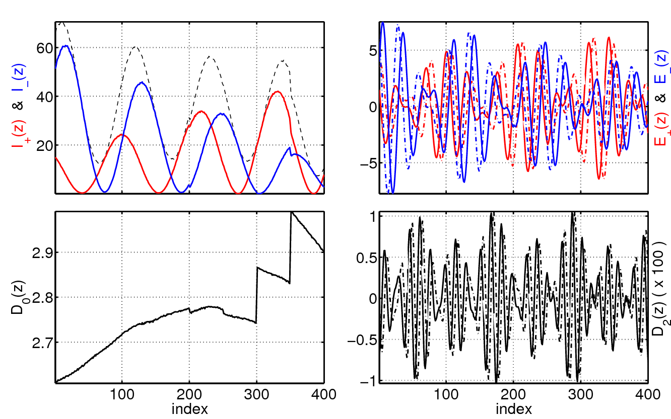
Current Modulation
One of the most direct way to transfer information into the output of a laser is to modulate the amplitude of the optical wave by varying the strength of the laser current excitation. Freetwm allows for arbitrary form of bias modulation, i.e. it is not limited to sinusoidal or square waveforms. Depending on the parameters of the modulation one can observe either a weakly non linear response or the onset of the so-called Q-switch regime. The latter case is depicted in the figure on the right where the laser emits bursts that exhibit a strongly multimode envelope evolving on the modal separation time scale. Another salient feature of the dynamics are the relaxation oscillation of the optical power around the frequency of 7 GHz. The bursts repetition rate of 1 GHz is controlled by the frequency of the bias current modulation and is easily identifiable in the power spectrum. Some simple routines based on Octave or Matlab fft routines allow to perform optical and power spectrum of the field and of its intensity, respectively.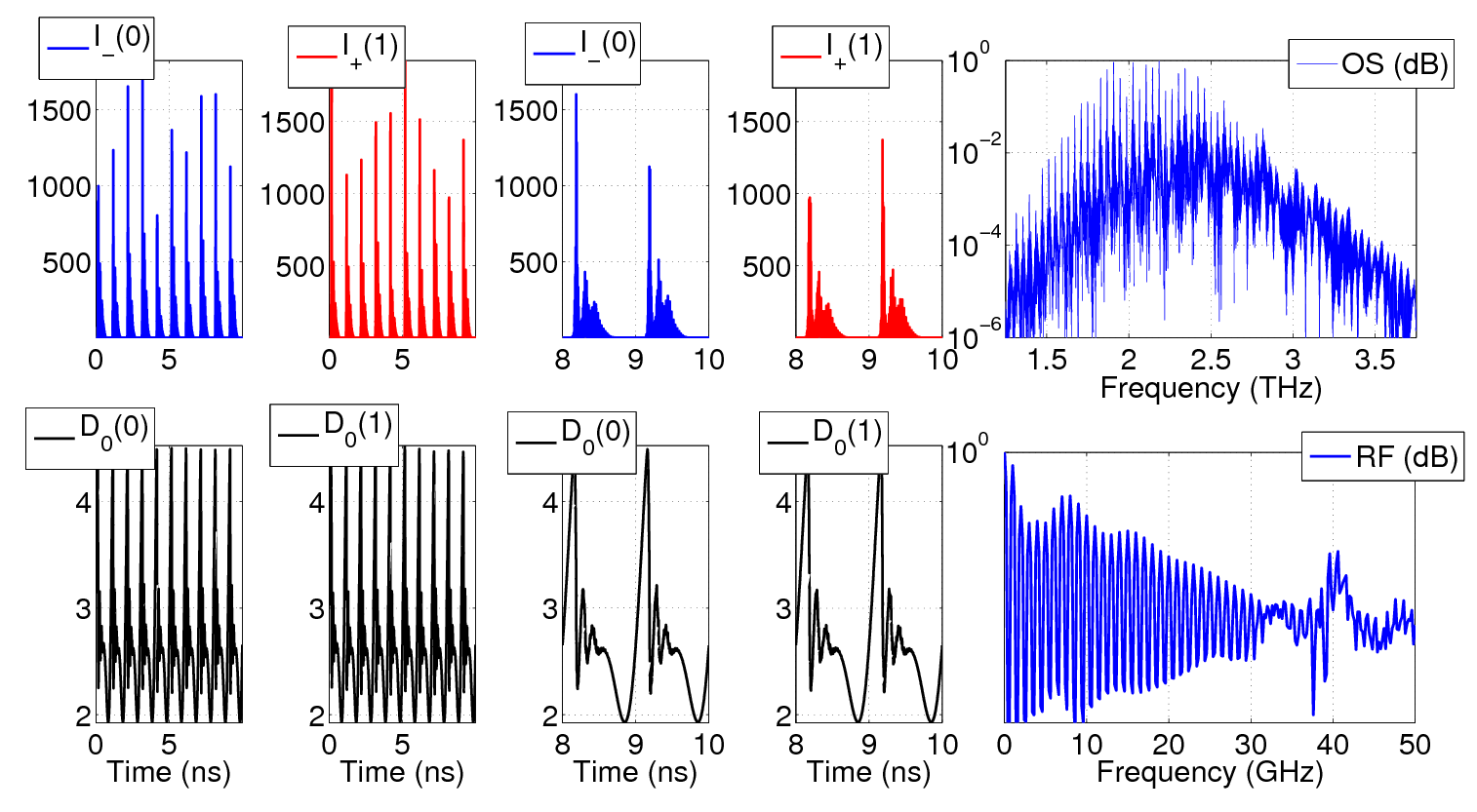
Voltage Modulation
Another efficient way to modulate an incoming optical signal is to use a saturable absorber based electro-optical modulator. Here, the imposed modulation of the reverse voltage induces a change in the band-gap frequency of the semiconductor material therefore modifying the amount of saturable absorption at the wavelength of the injected field. Freetwm can be used to study the optical response to an arbitrary modulation of the active medium band-gap. One can observe on the left the optical response of an absorber submitted to an 5 GHz sinusoidal modulation of its band-gap frequency. The incoming signal is 2 ns quasi-square pulse. Notice how such a few nanometers harmonic modulation of the band-gap give rise to a strongly non linear response with 100% modulation depth.
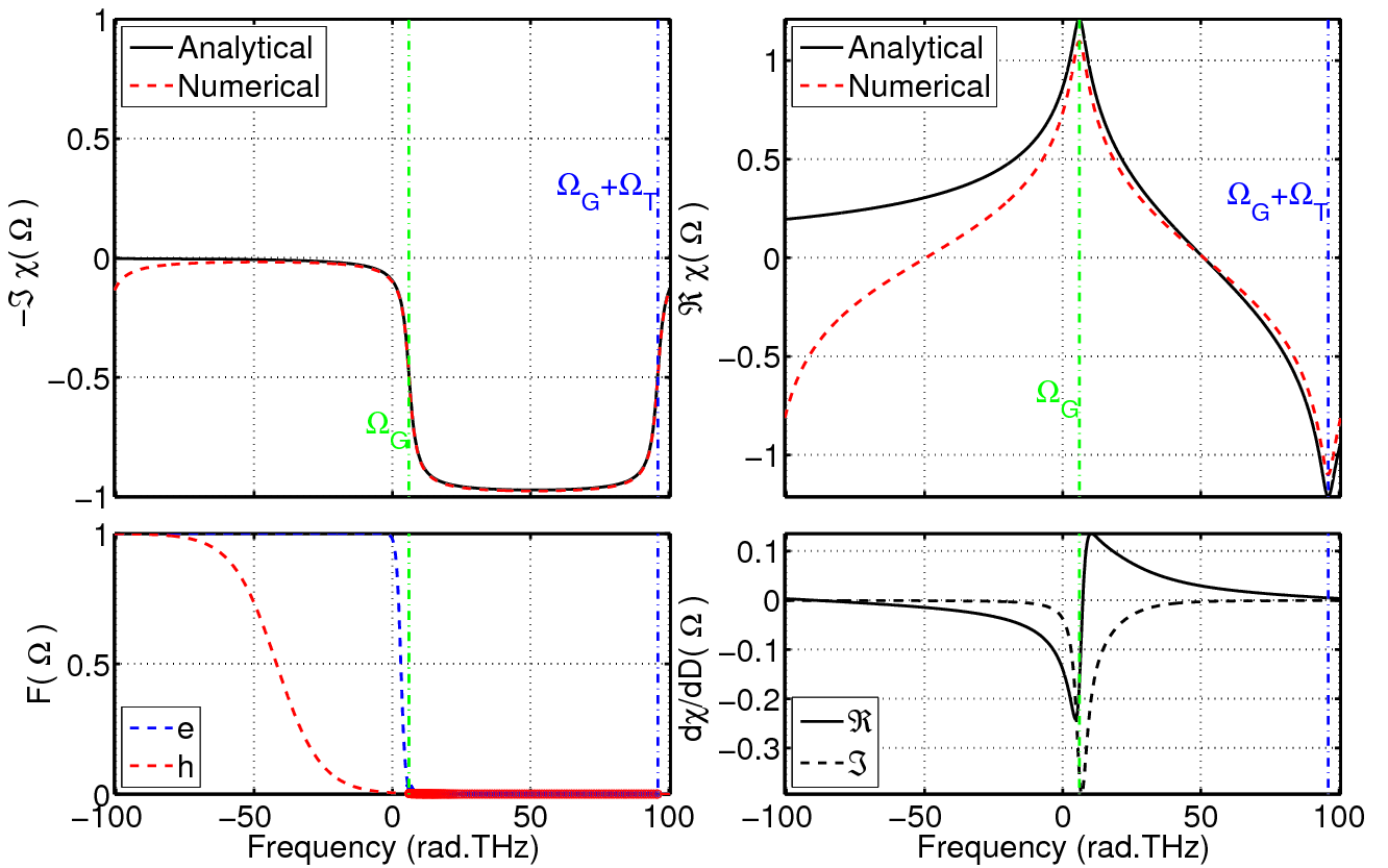
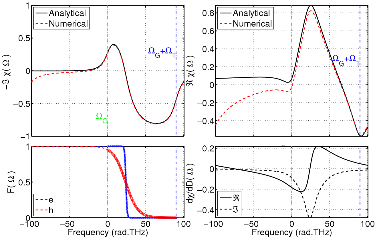
Material Response
The optical response is based on an analytical result for a two band Quantum Well assuming a quasi-equilibrium Fermi distribution of the electron and holes within the band [3,4]. No ad-hoc fitting with Lorentzian line shapes is needed. As such, this approach gives uniformly accurate results both for low carrier densities like e.g. for saturable absorbers (see below on the left where the Fermi levels are deep below the band-gap), and for high carrier densities like e.g. saturable Amplifiers, (see below on the right where the two Fermi levels are high within the band). Some functions in the toolbox allow to foresee the shape of the gain curve as a function of the material pare meters. In addition, a comparison between the exact gain and the “numerically stained” one is always given (see above in black and red) in order to keep the --unavoidable-- numerical problems related to aliasing and to the correct choice of the CFL [1] condition under control.